

R-squared nowadays is a strange metric that is not even mentioned in the ML community anymore because it is not used to evaluate modern ML models. However, understanding the intuition behind it and its proper interpretation is helpful to understand how noise in the data can impact model parameters. This post is from a white paper I wrote several years ago but I think it is still a good piece to reflect on how noise in the data can impact model parameters.
R-squared is a typical metric used to assess the performance of a Regression model. However, sometimes the analyst can experience model results with a very low R-squared value while coefficients statistically significant. Should the analyst proceed and trust the significant coefficients and ignore the low R-squared value? or Should the analysts discard completely the model?. This post try to address this apparent dilemma and provide some insights of how to face the challenge.
R-Squared is usually understood as the “percentage of variance explained” by the independent variables in the model. Since the definition is talking about explanatory power of the model to describe a “change” in the dependent variable, R-squared has a lot of implications on the prediction performance of the model. A low R-squared will mean a large residual standard error and a large confidence interval for prediction purposes while a high R-squared usually means small standard error and smaller confidence intervals for prediction which ultimately means more accurate ones.
Furthermore, these relationships are only relevant if Regression Assumptions are valid. In particular, the residual assumptions related with Normality, constant mean and constant variance.
One thing that is not so evident is that it is possible to capture accurately the linear model structure within a very noisy data set (low R-squared) if we are careful to validate that residuals comply with regression assumptions. However, if residuals are not complying with normality assumptions, a low R-squared can be a warning sign to the potential of capturing a complete different Linear model than the real one hiding behind the noise which ultimately can take the analyst to incorrect conclusions.
Let’s explore a few scenarios to understand the implications of Noise in R-squared and the model structure. First, I will demonstrate that if there exist an intrinsic Linear Pattern in the data and this model is affected by white noise, linear regression can still detect the linear model structure with strong confidence regardless of the R-squared value. Secondly, in contrast, I will show how noise that is not normal can trick the regression process to return an incorrect significant model.
A Linear Model + White Noise
To understand the meaning of the R-squared metric, let’s assume we have a line and add white noise to each point in the line to create a dataset of signal+noise. I will change the noise level to demonstrate that under this condition (i.e. strong underlying linear model + white noise) linear regression can return a valid model structure regardless of the R-squared value and noise level.
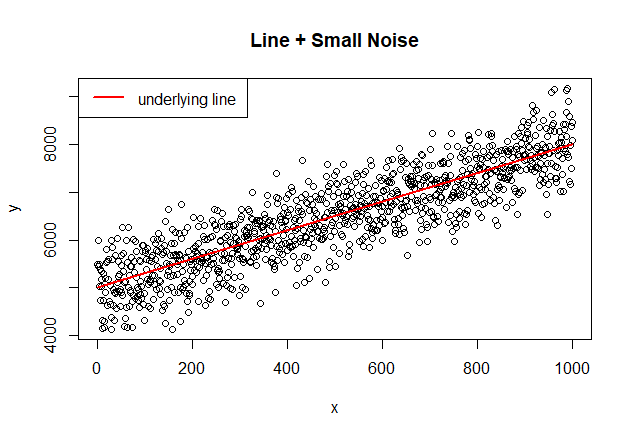
Linear Model Y= 5000 + 3X and Small White Noise
A good start is to look into a Linear Model with a small amount of White Noise. We should expect a good regression model.
# Creating a dataset of 1000 points from a normal distribution
set.seed(500)
noise_small<-rnorm(1000,0,500)
# adding Noise to the line Y=5000 + 3X
x<-seq(1:1000)
y<-noise_small+(5000+3*x)
line<-5000+3*x
# plot with the underlying model
plot(x,y, main="Line + Small Noise")
lines(line, col="red", lwd=2)
legend ("topleft", legend=c("underlying line"), col=c("red"), lty=1, lwd=2)
# Let's perform the regression...
data<-data.frame(x=x,y=y)
model<-lm(y ~ x, data)
summary(model)
##
## Call:
## lm(formula = y ~ x, data = data)
##
## Residuals:
##    Min     1Q Median     3Q    Max
##  -1332   -332      6    356   1387
##
## Coefficients:
##             Estimate Std. Error t value Pr(>|t|)
## (Intercept) 4.97e+03   3.16e+01   157.2   <2e-16 ***
## x           3.01e+00   5.47e-02    54.9   <2e-16 ***
## ---
## Signif. codes:  0 '***' 0.001 '**' 0.01 '*' 0.05 '.' 0.1 ' ' 1
##
## Residual standard error: 500 on 998 degrees of freedom
## Multiple R-squared:  0.751,  Adjusted R-squared:  0.751
## F-statistic: 3.02e+03 on 1 and 998 DF,  p-value: <2e-16
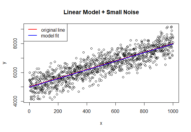
It is important to pay attention that the intercept and coefficient are 4972.0053, 3.0072 respectively. The model is fitting nicely the underlying line as reflected in the significant coefficients and the close match in the picture shown below. This result is what we would expect if the noise is really white noise.
plot(x,y, main="Linear Model + Small Noise")
lines(line, col="red", lwd=2)
lines(predict(model,data.frame(x=x)), col="blue", lwd=2)
legend ("topleft", legend=c("original line", "model fit"), col=c("red","blue"), lty=1, lwd=2)
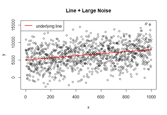
Linear Model Y= 5000 + 3X and Large White Noise
Now, Let’s compare how regression performs with a large White Noise component
set.seed(500)
noise_large<-rnorm(1000,0,3000)
# adding Noise to the line Y=5000 + 3X
x<-seq(1:1000)
y<-noise_large+(5000+3*x)
line<-5000+3*x
# plot with the underlying line
plot(x,y, main="Line + Large Noise")
lines(line, col="red", lwd=2)
legend ("topleft", legend=c("underlying line"), col=c("red"), lty=1, lwd=2, bg="white")
# Let's perform the regression...
data<-data.frame(x=x,y=y)
model<-lm(y ~ x, data)
summary(model)
##
## Call:
## lm(formula = y ~ x, data = data)
##
## Residuals:
##    Min     1Q Median     3Q    Max
##  -7989  -1993     36   2136   8324
##
## Coefficients:
##             Estimate Std. Error t value Pr(>|t|)
## (Intercept) 4832.032    189.777   25.46   <2e-16 ***
## x              3.043      0.328    9.27   <2e-16 ***
## ---
## Signif. codes:  0 '***' 0.001 '**' 0.01 '*' 0.05 '.' 0.1 ' ' 1
##
## Residual standard error: 3000 on 998 degrees of freedom
## Multiple R-squared:  0.0792, Adjusted R-squared:  0.0783
## F-statistic: 85.9 on 1 and 998 DF,  p-value: <2e-16
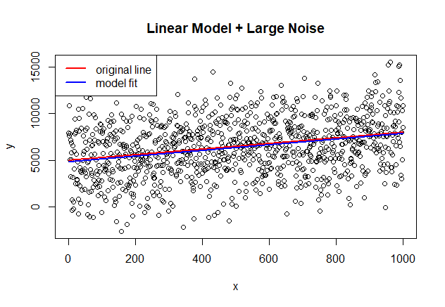
Notice how the coefficients (4832.0315, 3.0434) still fit very closely the original model parameters as reflected in the significant coefficients and the close match in the picture shown below. But what is more interesting is that the R-squared is degraded considerable (~ 8% with large noise vs ~75% with small noise). The analyst still can draw important conclusions from the coefficients of the model but probably can not use the model for prediction purposes because of the low R-squared and large standard error of the model which will put the predictions with a high level of uncertainty. This scenario is something I always verify in my ML models: if the error values of my model behave like white noise, then I know the model picked the "signal" from the data correctly and at least I know I can use my model for explanatory purposes.
A Linear Model and Non-White Noise…
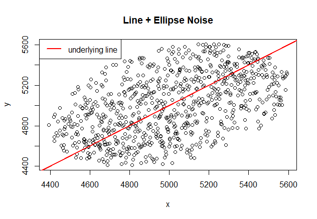
Now, assume we have a linear model Y=X and we add noise around the line but we constraint the noise to a shape of an ellipse that has one of its axles in the line Y=X as well. This time the noise will not be white noise as its distribution is altered. We will notice how things can go wrong here..
# the ellipse of noise will be centered at (5000,5000) but rotated 45 degrees to match
# the underlying linear model
angle<-pi/4
a<-700
b<-500
center_x <- 5000
center_y <- 5000
angle<-pi/4
data<-data.frame(x=seq(1:noisepoints),y=noisyaxle)
# filter noise points within the ellipse
points<-data[((data$x-center_x)*cos(angle)+(data$y-center_y)*sin(angle))^2/a^2 + (-(data$x-center_x)*sin(angle)+(data$y-center_y)*cos(angle))^2/b^2 <= 1,]
plot(points, main="Line + Ellipse Noise")
lines(seq(1:noisepoints),seq(1:noisepoints), col="red", lwd=2)
legend ("topleft", legend=c("underlying line"), col=c("red"), lty=1, lwd=2, bg="white")
# Executing the regression
model<-lm(y ~ x , points)
summary(model)
##
## Call:
## lm(formula = y ~ x, data = points)
##
## Residuals:
##    Min     1Q Median     3Q    Max
## -588.8 -214.2    0.5  200.9  575.8
##
## Coefficients:
##             Estimate Std. Error t value Pr(>|t|)
## (Intercept) 2.41e+03   1.58e+02    15.3   <2e-16 ***
## x           5.18e-01   3.16e-02    16.4   <2e-16 ***
## ---
## Signif. codes:  0 '***' 0.001 '**' 0.01 '*' 0.05 '.' 0.1 ' ' 1
##
## Residual standard error: 266 on 801 degrees of freedom
## Multiple R-squared:  0.251,  Adjusted R-squared:  0.251
## F-statistic:  269 on 1 and 801 DF,  p-value: <2e-16
This time the coefficients (2414.3008, 0.5176) are not capturing very well the underlying structure of the line Y=X. This is because of the weak directionality of the dataset imposed by the noise that “confuses” the regression process. The model coefficients are highly significant but the R-squared is considerable lower than in the previous case. This combination should trigger a warning sign to the analyst that should take the proper steps to verify residual assumptions. This model might not be a good model for either predicting “Y" or getting insights from the coefficients.
# Looking at the underlying line and model fit... not lucky this time...
plot(points, main="Line + Ellipse Noise")
lines(seq(1:noisepoints),seq(1:noisepoints), col="red", lwd=2) # the real axle
lines(seq(1:noisepoints),predict(model,data.frame(x=seq(1:noisepoints))), col="blue", lwd=2)
legend ("topleft", legend=c("original line", "model fit"), col=c("red","blue"), lty=1, lwd=2, bg="white")
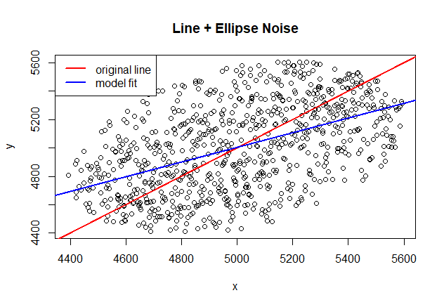
This is a good example where the combination of large noise (captured by the low R-squared value) and the violation of residual assumptions make the model unreliable for statistical insights even if the model and coefficients are significant.
Conclusion
is low R-squared a problem?. The answer is: “It depends”. The real answer is that as long as we verify Regression assumptions, in particular Residual assumptions, and use good judgment at the time of verifying them, we should be able to get insights from the significant coefficients of a regression model even if the R-squared is low. If assumptions are violated and R-squared is low then most probably the model is not reliable even with significant coefficients. The practical implication for ML practitioners is that we should also look at the properties of the error distributions to verify they are not showing any patterns that could mean our model did not capture the "signal" in the data. Buenas Noches!!